library(httr2)
library(dplyr)
library(jsonlite)
library(ggplot2)
library(sf)

req <- request("https://www.systembolaget.se/api/gateway/sitesearch/site/")
req <- req %>% req_headers("baseURL" = "https://api-systembolaget.azure-api.net/sb-api-ecommerce/v1")

# req_dry_run(req)
resp <- req_perform(req)
systembolaget_list <- jsonlite::fromJSON(resp_body_string(resp))

systembolaget_df <- bind_cols(
systembolaget_list$siteSearchResults %>%
  select(siteId,alias,city),
systembolaget_list$siteSearchResults$position
) %>%
  filter(!is.na(longitude),
         latitude >= 10)
systembolaget_sf <- sf::st_as_sf(systembolaget_df, coords = c("longitude","latitude"), crs = "EPSG:4326") %>%
  st_transform(crs = 3067) %>%
  mutate(store_name = as.character(siteId))

library(rvest)

html <- read_html("https://www.alko.fi/myymalat-palvelut/")

nayta_lisatiedot <- html %>%
  html_elements(".show-info") %>%
  html_attrs()

lista <- list()
for (i in seq(nayta_lisatiedot)){
  print(paste0(i, "/", length(nayta_lisatiedot)))
  html_lisatiedot <- read_html(nayta_lisatiedot[[i]][[1]])
  sijainti_lst <- html_lisatiedot %>%
    html_elements("meta") %>%
    html_attrs()

  for (ii in seq(sijainti_lst)){
    if (any(grepl("property", names(sijainti_lst[[ii]])))){
      # Lets pick the name
      if (sijainti_lst[[ii]][[1]] == "og:title"){
        name <- sijainti_lst[[ii]][[2]]
      }
      # lets pick the location
      if (sijainti_lst[[ii]][[1]] == "og:image"){
        loc <- strsplit(gsub("^.+center=|&size.+$", "", sijainti_lst[[ii]][[2]]), split = ",") |> unlist()
      }
      # lets pick the location
      if (sijainti_lst[[ii]][[1]] == "og:image"){
        loc <- strsplit(gsub("^.+center=|&size.+$", "", sijainti_lst[[ii]][[2]]), split = ",") |> unlist()
      }
    } else next()
  }
  lista[[i]] <- tibble(name = name, lat = loc[1], lng = loc[2])
  rm(name)
  rm(loc)
}
alko_sf <- do.call("bind_rows", lista) %>%
  sf::st_as_sf(coords = c("lng","lat"), crs = "EPSG:4326") %>%
  mutate(type = ifelse(grepl("Noutopiste", name), "take-away", "store"))

alko_sf_store <- alko_sf %>%
  filter(type == "store") %>%
  mutate(store_name = name) %>%
  st_transform(crs = 3067)

# Plot the store locations
stores_swe_fin <- rbind(alko_sf_store %>% select(store_name),
                    systembolaget_sf %>% select(store_name)) %>%
  mutate(bolag = ifelse(grepl("alko|Alko", store_name), "Alko", "Systembolaget"))

alko_swe_fin_plot <- ggplot() +
  geom_sf(data = stores_swe_fin, aes(color = bolag), shape = 21) +
  scale_color_manual(values = c("#e31c18", "#00813c")) +
  labs(title = "Government-owned liquor store locations in Finland (Alko) and \nSweden (Systembolaget",
       color = NULL)
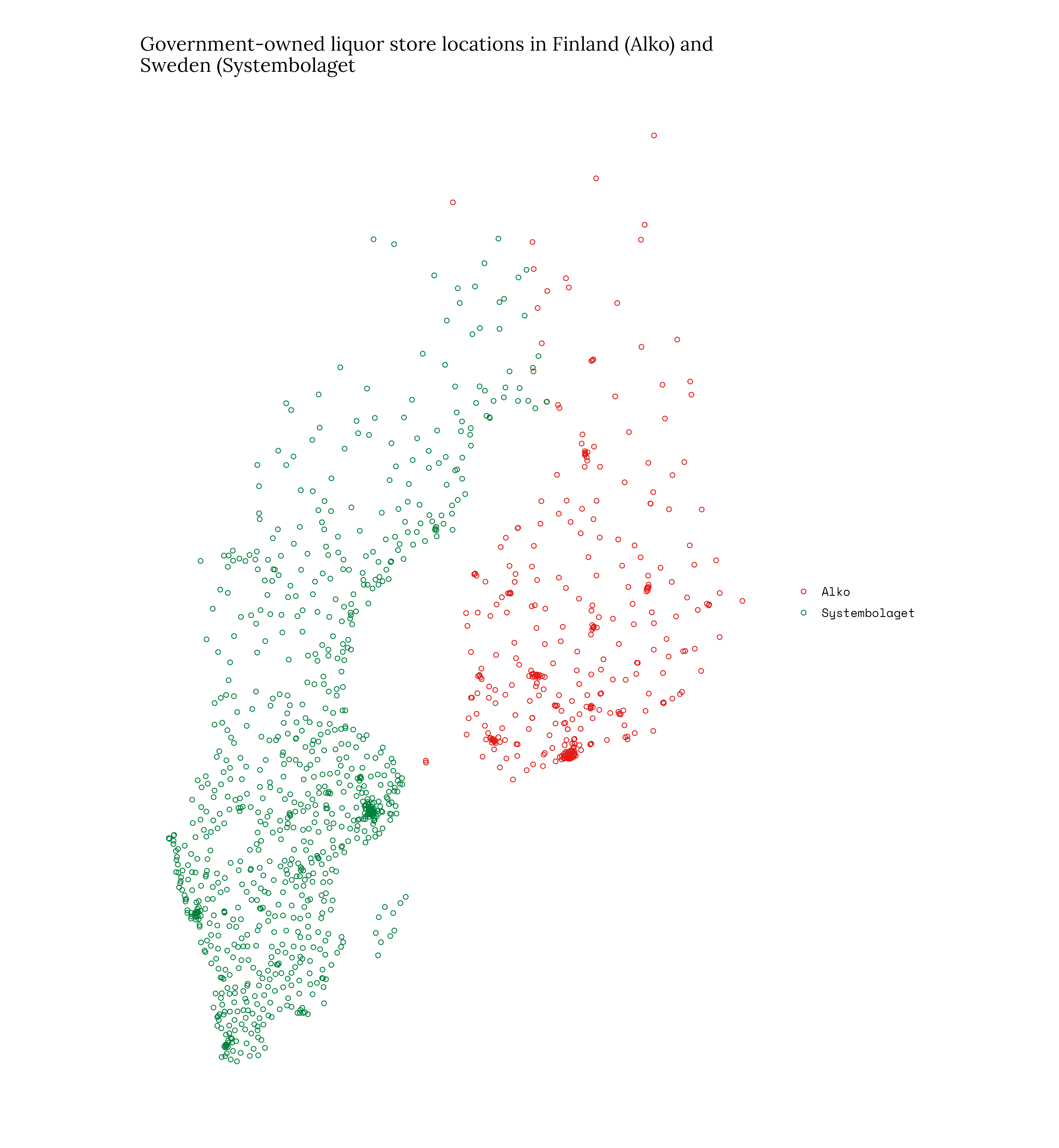
alko_swe_fin_plotThis is not a study, but another technical demo on how to use data from websites and proper spatial data sources in R programming language. Vague research question that I am looking to answer is “In which county, Sweden or Finland, people have better access to state liquor stores”.
In case you are only interested in the answer, by no surprise, the state supply of also alcohol is better taken care in Sweden. The mean distance to nearest liquor store by road in Sweden is 4.50km, whereas in Finland you have to ride your bicycle more than a kilometer longer. Mean distance in Finland is 5.95km.
Introduction
These two countries are chosen because they both have a state monopoly in alcohol retail, Alko in Finland and Systembolaget in Sweden.
Also, you there is population grid data openly available from both countries, at Statistics Finland and at Statistics Sweden.
Liquor store location data
To get the locations of liquor stores you need to apply http GETqueries in the case of Systembolaget and do shady web scraping in the case of Alko in Finland. Point coordinates are in WGS84 coordinate reference system by default that you need to transform into ESPG:3067 which isthe projected coordinate system for Finland that I use here.

Population grid data
For Finnish data you can use functions from geofi-package. Statistics Sweden disseminates spatial data in geopackage-format. Just download the zipped file, unzipt and read to R.
# Finland
grid_finland <- geofi::get_population_grid(resolution = 1) %>%
  mutate(grid_id = id_nro)

# Sweden
tmpfly <- tempfile()
tmpdir <- tempdir()
download.file("https://www.scb.se/contentassets/67248cebde154e009c3bee2ee01dca35/totalbefolkning_1km_211231.zip", tmpfly)
unzip(zipfile = tmpfly, exdir = tmpdir)
filename <- grep("gpkg", fs::dir_ls(tmpdir), value = TRUE)
grid_sweden_espg3067 <- sf::st_read(filename, crs = 3006) %>%
  sf::st_transform(crs = 3067) %>%
  mutate(vaesto = Pop,
         grid_id = Ruta
)
# grid
grid_swe_fin <- rbind(grid_finland %>% select(vaesto),
                      grid_sweden_espg3067 %>% select(vaesto))

grid_swe_fin_plot <- ggplot() +
  geom_sf(data = grid_swe_fin, aes(fill = vaesto), color = NA) + scale_fill_viridis_b() +
  labs(title = "Population by 1x1km grid in Finland and Sweden", fill = "Population \nper cell")
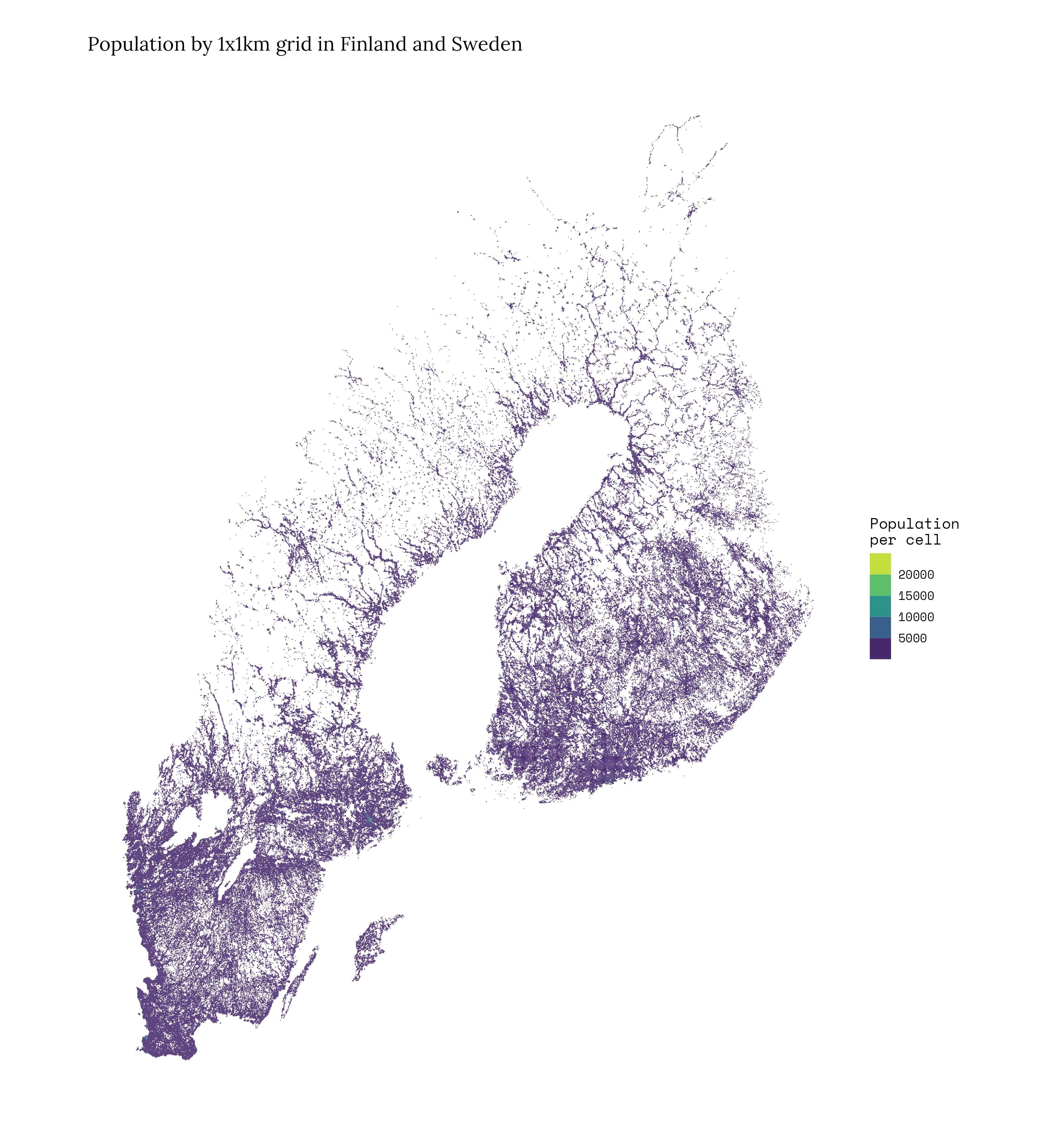
grid_swe_fin_plot
Distances between grid cells and stores
Computing distance between to points or to sets of points is straightforward and quick in R. We do this because later on, we only want to compute routes to nearest store to save time and electricity.
library(osrm)
library(dplyr)
library(sf)
library(geofi)

# Finland
stores_fin <- alko_sf_store
# grid data into centroids (points)
population_grid_fin <- grid_finland %>%
  st_centroid()

# distances as crow flies
dists <- st_distance(x = population_grid_fin, y = stores_fin)

dist_list <- list()
for (i in 1:nrow(dists)){
  if (i%%1000 == 0) print(paste0(i,"/",nrow(dists)))
  dist_list[[i]] <- tibble(store_name = stores_fin$store_name,
         distance = dists[i,]) %>%
    mutate(grid_id = population_grid_fin$grid_id[i])
}
dist_df_fin <- as.data.frame(data.table::rbindlist(dist_list))

dist_df_fin_shortest <- dist_df_fin %>%
  mutate(distance = as.numeric(distance)) %>%
  group_by(grid_id) %>%
  filter(distance == min(distance)) %>%
  ungroup() %>%
  left_join(st_drop_geometry(population_grid_fin))

# compute the mean distance per person
tot_dist <- dist_df_fin_shortest %>%
  summarise(total_distance = distance/1000 * vaesto) %>%
  summarise(total_distance = sum(total_distance))
tot_pop <- dist_df_fin_shortest %>%
  summarise(total_population = sum(vaesto))
mean_dist_fin <- tot_dist/tot_pop
# 4.178743
# Sweden
stores_swe <- systembolaget_sf
# grid data into centroids (points)
population_grid_swe <- grid_sweden_espg3067 %>%
st_centroid()
# distances as crow flies
dists <- st_distance(x = population_grid_swe, y = stores_swe)
dist_list <- list()
for (i in 1:nrow(dists)){
if (i%%1000 == 0) print(paste0(i,"/",nrow(dists)))
dist_list[[i]] <- tibble(store_name = stores_swe$store_name,
distance = dists[i,]) %>%
mutate(grid_id = population_grid_swe$grid_id[i])
}
dist_df_swe <- as.data.frame(data.table::rbindlist(dist_list))
dist_df_shortest_swe <- dist_df_swe %>%
mutate(distance = as.numeric(distance)) %>%
group_by(grid_id) %>%
filter(distance == min(distance)) %>%
ungroup() %>%
left_join(st_drop_geometry(population_grid_swe))
# compute the mean distance per person
tot_dist <- dist_df_shortest_swe %>%
summarise(total_distance = distance/1000 * vaesto) %>%
summarise(total_distance = sum(total_distance))
tot_pop <- dist_df_shortest_swe %>%
summarise(total_population = sum(vaesto))
mean_dist_swe <- tot_dist/tot_pop
# 2.932753As we have now calculated the as-crow-flies distances, we can conclude that that Swedes only have to fly, on average, 2.93 km to get their bottle of Absolut, while Finns need to take a lot longer flight of 4.18 km for their Koskenkorva.
But as a drunk people are not allowed to fly, we need to calculate the distances by road that they can walk. Here we assume, that the nearest alcohol store by flying would be the nearest also by road, we only do routing for these trips. (This is not the case for instance in the Archipelago!)
Routing through road network using Open Source Routing Machine (OSRM)
For routing we could use a commercial routing APIs like Google or Yahoo, but let’s rather create our own for the sake of privacy, speed and costs. Learn Open Source Routing Machine if you haven’t already.
Configure OSRM Docker containers
For the routing exercise you need to have docker installed and some file download utility, I use wget here. The docker commands below are meant to run in os terminal, not in R!
First prepare the OSRM containers for both countries.
# Download the background image
docker pull osrm/osrm-backend
# Tag different version for Finland and Sweden
docker tag osrm/osrm-backend osrm-backend:finland
docker tag osrm/osrm-backend osrm-backend:sweden

## Finland

# Download latest road network from OpenStreetMap
wget http://download.geofabrik.de/europe/finland-latest.osm.pbf

# extract
docker run -t -v "${PWD}:/data" osrm-backend:finland osrm-extract -p /opt/car.lua /data/finland-latest.osm.pbf
# partition
docker run -t -v "${PWD}:/data" osrm-backend:finland osrm-partition /data/finland-latest.osrm
# customize
docker run -t -v "${PWD}:/data" osrm-backend:finland osrm-customize /data/finland-latest.osrm


## Sweden

# Download latest road network from OpenStreetMap
wget http://download.geofabrik.de/europe/sweden-latest.osm.pbf

# extract
docker run -t -v "${PWD}:/data" osrm-backend:sweden osrm-extract -p /opt/car.lua /data/sweden-latest.osm.pbf
# partition
docker run -t -v "${PWD}:/data" osrm-backend:sweden osrm-partition /data/sweden-latest.osrm
# customize
docker run -t -v "${PWD}:/data" osrm-backend:sweden osrm-customize /data/sweden-latest.osrm
The start the two containers before you fire up the routing in the R code below.
## Launch Finland
docker run -t -i -p 5000:5000 -v "${PWD}:/data" osrm-backend:finland osrm-routed --algorithm mld /data/finland-latest.osrm
## Launch Sweden
docker run -t -i -p 5001:5000 -v "${PWD}:/data" osrm-backend:sweden osrm-routed --algorithm mld /data/sweden-latest.osrm
Run the routing
Once the containers are waiting for requests, let’s run the R code below to get the distances and routes along the roads.
# swe
destination <- stores_swe %>%
  right_join(dist_df_shortest_swe)
origin <- population_grid_swe %>%
  right_join(dist_df_shortest_swe)

options(osrm.server = "http://127.0.0.1:5001/")

origins <- unique(origin$Ruta)
list1 <- list()
for (i in seq(origins)){
  if (i%%100 == 0) print(paste0(i,"/",length(origins)))

  tmp_res <- osrmRoute(src = origin[origin$Ruta %in% origins[i],],
                       dst = destination[destination$grid_id %in% origins[i],],
                       overview = "simplified"
                       )
    list1[[i]] <- tmp_res %>%
      mutate(
        grid_id = origins[i],
        store_name = stores_swe$name[i]
                           )
  }
df_routes_swe <- as.data.frame(data.table::rbindlist(list1))
lines_swe <- df_routes_swe$geometry
lines_swe_sf <- sf::st_as_sf(lines_swe)
lines_swe_sf <- cbind(lines_swe_sf,df_routes_swe %>% select(-geometry))


# fin
dist_df_shortest_fin <- readRDS("dist_df_fin_shortest.RDS")
destination <- stores_fin %>%
  right_join(dist_df_shortest_fin)
origin <- population_grid_fin %>%
  right_join(dist_df_shortest_fin)

options(osrm.server = "http://127.0.0.1:5000/")
origins <- unique(origin$grid_id)
list1 <- list()
for (i in 11567:length(origins)){
# for (i in seq(origins)){
  if (i%%100 == 0) print(paste0(i,"/",length(origins)))

  tmp_res <- osrmRoute(src = origin[origin$grid_id %in% origins[i],],
                    dst = destination[destination$grid_id %in% origins[i],],
                    overview = "simplified"
                    )
    list1[[i]] <- tmp_res %>%
      mutate(
        grid_id = origins[i],
        store_name = stores_fin$name[i]                           )
  }

df_routes_fin <- as.data.frame(data.table::rbindlist(list1))
lines_fin <- df_routes_fin$geometry
lines_fin_sf <- sf::st_as_sf(lines_fin)
lines_fin_sf <- cbind(lines_fin_sf,df_routes_fin %>% select(-geometry))
It took some time, but we are ready now. What are the mean distances along roads then?
# For Finland
d_tot_road <- left_join(df_routes_fin, grid_finland)

tot_dist <- d_tot_road %>%
  summarise(total_distance = distance * vaesto) %>%
  summarise(total_distance = sum(total_distance))
tot_pop <- d_tot_road %>%
  summarise(total_population = sum(vaesto))
mean_dist_fin_road <- tot_dist/tot_pop
mean_dist_fin_road
# 5.945485

# For Sweden
d_tot_road <- left_join(df_routes_swe, grid_sweden_espg3067)

tot_dist <- d_tot_road %>%
  summarise(total_distance = distance * vaesto) %>%
  summarise(total_distance = sum(total_distance))
tot_pop <- d_tot_road %>%
  summarise(total_population = sum(vaesto))
mean_dist_swe_road <- tot_dist/tot_pop
mean_dist_swe_road
# 4.499895
Results
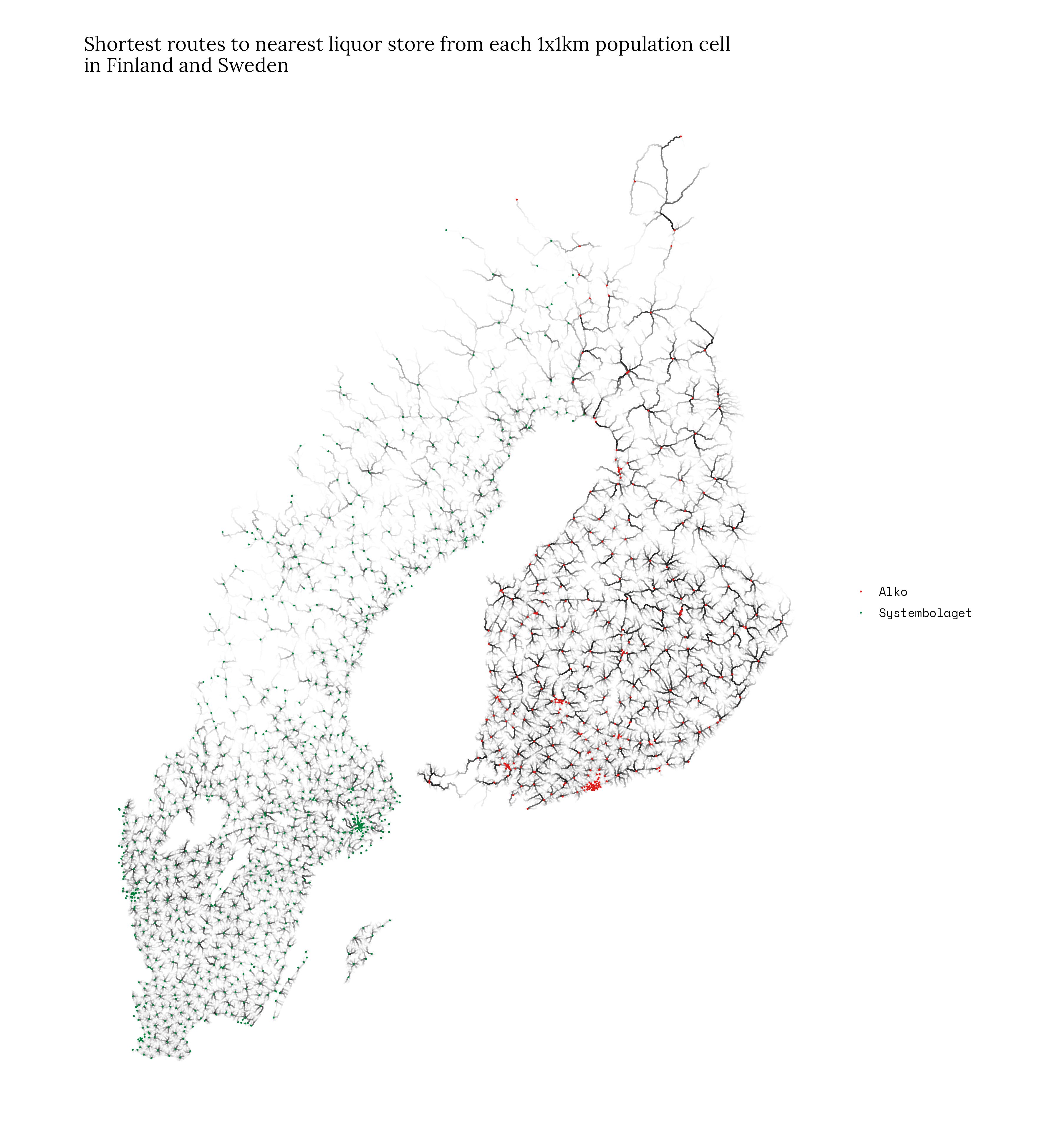
As stated at the beginning, Swedes live slightly closer to liquor stores, on average, than Finns. 4.499895 kilometers vs. 5.945485 kilometers.
Let’s create the final plot, with the shortest routes and the liquor stores combined with the following code.
lines_both <- rbind(lines_swe_sf %>% select(distance),
                    lines_fin_sf %>% select(distance))


routes_both <- ggplot(lines_both #%>% sample_n(size = 100000)
                      ) +
  geom_sf(alpha = .01) +
  geom_sf(data = stores_swe_fin, aes(color = bolag), size = .1) +
  scale_color_manual(values = c("#e31c18", "#00813c")) +
  labs(title = "Shortest routes to nearest liquor store from each 1x1km population cell \nin Finland and Sweden",
       color = NULL)
routes_both
Click to a larger version
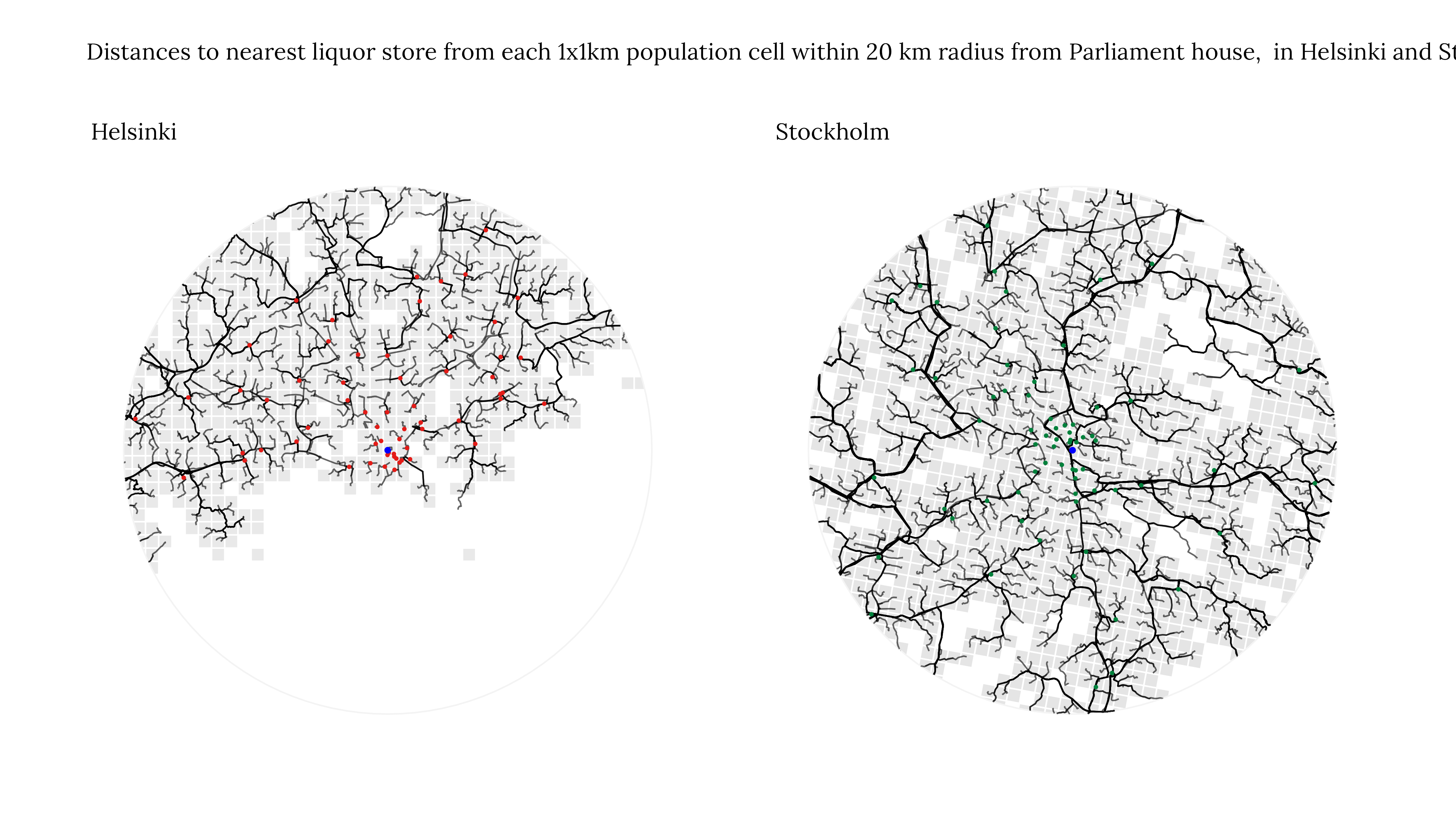
Extra: Stockholm and Helsinki
Lets also plot similar maps of the capital cities, ie. 20 km boundaries around the parliament houses. Coordinates are easy to find from Wikipedia articles: Riksdag and Parliament of Finland.
parliament_fin <- tibble(lon = 24.933333, lat = 60.1725) %>%
  sf::st_as_sf(coords = c("lon","lat"), crs = 4326) %>%
  st_transform(3067)
parliament_swe <- tibble(lon = 18.0675, lat = 59.3275) %>%
  sf::st_as_sf(coords = c("lon","lat"), crs = 4326) %>%
  st_transform(3067)

parliament_fin_buf <- st_buffer(x = parliament_fin, dist = 20000)
parliament_swe_buf <- st_buffer(x = parliament_swe, dist = 20000)


p1 <- ggplot() +
  geom_sf(data = grid_finland %>% st_intersection(parliament_fin_buf), color = "white", fill = alpha("grey", 1/3)) +
  geom_sf(data = lines_fin_sf %>% st_intersection(parliament_fin_buf), alpha = .6) +
  geom_sf(data = alko_sf_store %>% st_intersection(parliament_fin_buf), color = "#e31c18", size = .8) +
  geom_sf(data = parliament_fin, color = "blue") +
  geom_sf(data = parliament_fin_buf, color = alpha("grey", 1/6), fill = NA) +
  labs(title = "Helsinki")

p2 <- ggplot() +
  geom_sf(data = grid_sweden_espg3067 %>% st_intersection(parliament_swe_buf), color = "white",  alpha("grey", 1/3)) +
  geom_sf(data = lines_swe_sf %>% st_intersection(parliament_swe_buf), alpha = .6) +
  geom_sf(data = systembolaget_sf %>% st_intersection(parliament_swe_buf), color = "#00813c", size = .8) +
  geom_sf(data = parliament_swe, color = "blue") +
  geom_sf(data = parliament_swe_buf, color = alpha("grey", 1/6), fill = NA) +
  labs(title = "Stockholm")

p3 <- patchwork::wrap_plots(list(p1,p2), widths = c(1,1)) + patchwork::plot_annotation(title = "Distances to nearest liquor store from each 1x1km population cell within 20 km radius from Parliament house,  in Helsinki and Stockholm")
Reuse
Citation
@online{kainu2023,
  author = {Kainu, Markus},
  title = {Who Lives Closest to Liquor Store, {Finns} or {Swedes?}},
  date = {2023-01-17},
  url = {https://markuskainu.fi/posts/2023-01-18-alko-systembolaget/},
  langid = {en}
}