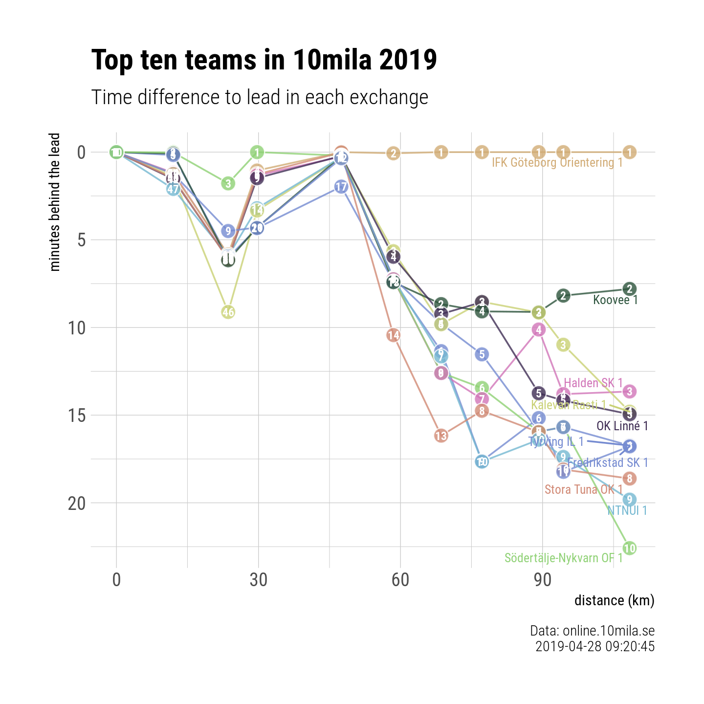
A Swedish spring classic in orienteering 10mila was raced this weeked in Östra Göinge in Skåne. Similar to last two years, IFK Göteborg won the mens 10 leg overnight relay. I took a little stab at their results system at online.10mila.se/, pulled out the data and did two graphs. You can download the excel data with two sheets from here: 10mila leg times & split times. I included the source code in R in case someone is interested in it.
Here are the positions for top 10 teams at each exchange!
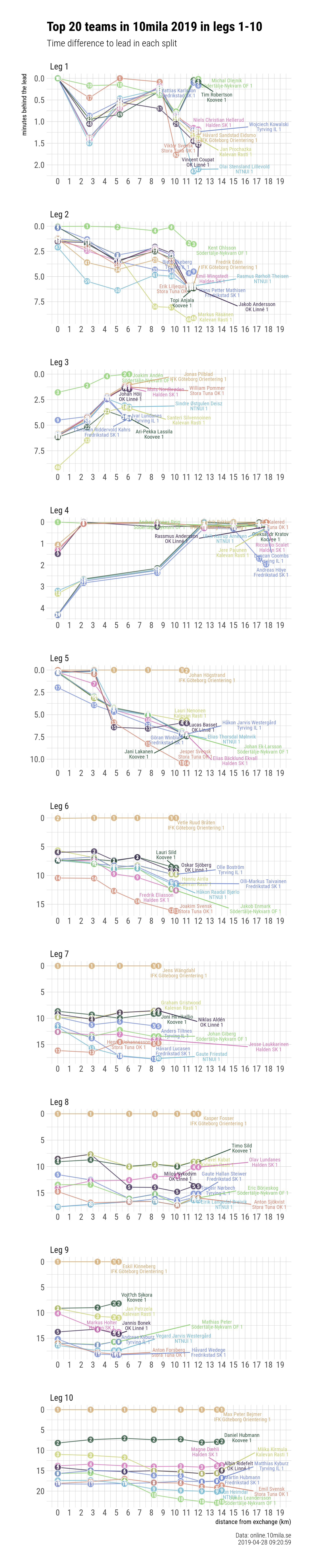
And below a very tall image with positions at each split point at each leg.
Source code
Is below.
[/kode]
library(httr)library(rvest)library(dplyr)osuus <-10looptbl <-data_frame(leg =1:10,splits =list(list(1,2,3,4,5), # 1list(1,2,3,4,5), # 2list(1,2,3), # 3list(1,2,3,4,5), # 4list(1,2,3,4), # 5list(1,2,3,4), # 6list(1,2,3), # 7list(1,2,3,4,5), # 8list(1,2), # 9list(1,2,3,4,5,6)) # 10)if (!file.exists("./data/osuusdata19.RDS")){# **********************************************************# vaihtoajatd_leg <-data_frame()for (leg in1:osuus){# for (leg in 1:10){read_html(paste0("http://online.10mila.se/index2.php?classId=1&legNo=",leg)) %>%html_table(fill =TRUE) %>% .[[5]] %>% .[-1:-2,] %>%as_tibble() -> tmpnames(tmp) <-c("place","name","club","time","diff") tmp$leg <- leg d_leg <-bind_rows(d_leg,tmp)}d_leg %>%mutate(min =as.integer(sub(":.+$", "", time)),s =as.integer(sub("^.+:", "", time)),secs = min *60+ s,diff_min =as.integer(sub(":.+$", "", diff)),diff_s =as.integer(sub("^.+:", "", diff)),diff_secs = diff_min *60+ diff_s ) -> d_leg2saveRDS(d_leg2, "./data/osuusdata19.RDS")}d_leg2 <-readRDS("./data/osuusdata19.RDS")leg_info <-data_frame(leg =1:10)leg_info %>%mutate(length =case_when( leg ==1~12.0, leg ==2~11.6, leg ==3~6.1, leg ==4~17.8, leg ==5~11.0, leg ==6~10.1, leg ==7~8.6, leg ==8~12.0, leg ==9~5.2, leg ==10~14.0), length_cum =cumsum(length)) -> leg_infod_leg22 <-left_join(d_leg2,leg_info)d_leg_0 <- d_leg22 %>%filter(leg == osuus) %>%mutate(length_cum =0, diff_secs =0,leg =0)d_leg_11 <-bind_rows(d_leg_0, d_leg22)all_legs <- d_leg_11 # for exceltop10 <- d_leg2 %>%filter(leg == osuus) %>%slice(1:10) %>%pull(club)d_leg_111 <- d_leg_11 %>%filter(club %in% top10)ipsum_palette <-c("#d18975", "#8fd175", "#3f2d54", "#75b8d1", "#2d543d", "#c9d175", "#d1ab75", "#d175b8", "#758bd1")ipsum_palette <-c(ipsum_palette,ipsum_palette,ipsum_palette)library(ggplot2)library(hrbrthemes)library(viridis)ggplot(d_leg_111, aes(x = length_cum, y = diff_secs/60, color = club, fill = club)) +geom_line(alpha = .8) +geom_point(shape =21, color ="white", alpha = .8, size =4) +# scale_x_continuous(breaks = leg_info$length_cum , labels = leg_info$leg) + scale_y_reverse() +geom_text(aes(label = place), color ="white", family ="Roboto Condensed", size =2.5, fontface="bold") +theme_ipsum_rc() + ggrepel::geom_text_repel(data = d_leg_111 %>%filter(leg ==max(leg)), aes(label = club), nudge_y =-.2, size =2.7, family ="Roboto Condensed") +theme(legend.position ="none") +# scale_fill_ipsum() + scale_color_ipsum() +scale_fill_manual(values =c(rev(ipsum_palette),"black")) +scale_color_manual(values =c(rev(ipsum_palette),"black")) +labs(title ="Top ten teams in 10mila 2019",subtitle ="Time difference to lead in each exchange",caption =paste0("Data: online.10mila.se\n",Sys.time()),x ="distance (km)", y ="minutes behind the lead") -> plotplot# **********************************************************# väliajatif (!file.exists("./data/valiaikadata.RDS")){d_splits <-data_frame()for (leg in1:osuus){# for (leg in 1:10){ splits <-unlist(looptbl$splits[leg]) split_dat <-data_frame()for (split1 in splits){read_html(paste0("http://online.10mila.se/index2.php?classId=1&legNo=",leg,"&splitNo=",split1)) %>%html_table(fill =TRUE) %>% .[[5]] %>% .[-1:-2,] %>%as_tibble() -> tmpnames(tmp) <-c("place","name","club","time","diff") tmp$leg <- leg tmp$split1 <- split1 split_dat <-bind_rows(split_dat,tmp)} d_splits <-bind_rows(d_splits,split_dat)}d_splits %>%mutate(min =as.integer(sub(":.+$", "", time)),s =as.integer(sub("^.+:", "", time)),secs = min *60+ s,diff_min =as.integer(sub(":.+$", "", diff)),diff_s =as.integer(sub("^.+:", "", diff)),diff_secs = diff_min *60+ diff_s ) -> d_splits2saveRDS(d_splits2, "./data/valiaikadata19.RDS")}d_splits2 <-readRDS("./data/valiaikadata19.RDS")split_info <- d_splits2 %>%count(leg,split1) %>%select(-n)split_info %>%mutate(length =case_when( leg ==1& split1 ==1~2.7, leg ==1& split1 ==2~5.3, leg ==1& split1 ==3~8.7, leg ==1& split1 ==4~10.1, leg ==1& split1 ==5~11.6, leg ==2& split1 ==1~2.5, leg ==2& split1 ==2~5.1, leg ==2& split1 ==3~8.3, leg ==2& split1 ==4~9.7, leg ==2& split1 ==5~11.2, leg ==3& split1 ==1~2.5, leg ==3& split1 ==2~4.2, leg ==3& split1 ==3~5.7, leg ==4& split1 ==1~2.2, leg ==4& split1 ==2~8.5, leg ==4& split1 ==3~12.5, leg ==4& split1 ==4~15, leg ==4& split1 ==5~17.2, leg ==5& split1 ==1~3.1, leg ==5& split1 ==2~4.8, leg ==5& split1 ==3~7.7, leg ==5& split1 ==4~10.6, leg ==6& split1 ==1~3.1, leg ==6& split1 ==2~4.8, leg ==6& split1 ==3~6.8, leg ==6& split1 ==4~9.7, leg ==7& split1 ==1~2.9, leg ==7& split1 ==2~5.3, leg ==7& split1 ==3~8.2, leg ==8& split1 ==1~2.8, leg ==8& split1 ==2~6.1, leg ==8& split1 ==3~8.3, leg ==8& split1 ==4~10.2, leg ==8& split1 ==5~11.6, leg ==9& split1 ==1~3.4, leg ==9& split1 ==2~4.8, leg ==10& split1 ==1~2.8, leg ==10& split1 ==2~5.7, leg ==10& split1 ==3~8.2, leg ==10& split1 ==4~10.5, leg ==10& split1 ==5~12.3, leg ==10& split1 ==6~13.6 )) %>%group_by(leg) %>%mutate(length_cum =cumsum(length)) -> split_infod_splits_10 <-left_join(d_splits2,split_info)d_leg0 <- all_legs %>%filter(leg %in%1:osuus) %>%mutate(length =0, diff_secs =0,leg =1)if (exists("d_leg_10")){d_leg_11 <-bind_rows(all_legs, d_leg_10) } else {d_leg_11 <- all_legs }d_leg_11_0 <- d_leg_11 %>%mutate(length =0, leg = leg +1)legdata <-bind_rows(d_leg_11,d_leg_11_0)d_splits_10 <-bind_rows(d_splits_10,legdata)d_splits_10 <- d_splits_10 %>%filter(leg !=0, leg !=11)d_splits_10$leg2 <-paste0("Leg ", d_splits_10$leg)d_splits_10$leg2 <-factor(d_splits_10$leg2, levels =c("Leg 1","Leg 2","Leg 3","Leg 4","Leg 5","Leg 6","Leg 7","Leg 8","Leg 9","Leg 10"))all_splits <- d_splits_10 # exceliind_splits_10 <- d_splits_10 %>%filter(club %in% top10)library(ggplot2)library(hrbrthemes)library(viridis)d_splits_10 <- d_splits_10 %>%filter(leg %in%1:osuus)ggplot(d_splits_10, aes(x = length, y = diff_secs/60,# y = diff_secs, color = club, fill = club)) +geom_line(alpha = .8) +geom_point(shape =21, color ="white", alpha = .8, size =4) + ggrepel::geom_text_repel(data = d_splits_10 %>%group_by(leg2) %>%filter(length ==max(length)), aes(label =paste0(name,"\n",club)), nudge_y =-.2, nudge_x =1, size =2.6, lineheight = .8, family ="Roboto Condensed") +facet_wrap(~leg2, ncol =1, scales ="free") +# scale_x_continuous(breaks = 0:18, labels = 0:18, limits = c(0,18)) +scale_x_continuous(breaks =0:19, labels =0:19, limits =c(0,19)) +scale_y_reverse() +geom_text(aes(label = place), color ="white", family ="Roboto Condensed", size =2.5, fontface="bold") +theme_ipsum_rc() +theme(legend.position ="none") +scale_fill_manual(values =c(rev(ipsum_palette),"black")) +scale_color_manual(values =c(rev(ipsum_palette),"black")) +# theme(plot.margin = unit(0,0,0,0)) +# theme(margin(t = 0, r = 0, b = 0, l = 0, unit = "pt")) +labs(title = glue::glue("Top 20 teams in 10mila 2019 in legs 1-{osuus}"),subtitle ="Time difference to lead in each split",caption =paste0("Data: online.10mila.se\n",Sys.time()),x ="distance from exchange (km)", y ="minutes behind the lead") -> splitspic