Quick and dirty analysis of 10mila 2018 results

A Swedish spring classic in orienteering 10mila was raced this weeked in Nynäshamn south of Stockholm. Similar to last year, IFK Göteborg won the mens 10 leg overnight relay and I took part totally unprepared. I took a little stab at their results system at online.10mila.se/, pulled out the data and did three graphs from it. You can download the data in two sheet excel from here: 10mila leg times & split times. I included the source code in R in case someone is interested in it. But without any styling or documentation!

Suomeksi pari sanaa. 10milan reissu kohta tehty ja ajan tappamiseksi kirjoittelin paluumatkalla koodia, miten hakea dataa 10milan tulospalvelusta ja analysoida sitä itse. Koodi on R-kieltä.

Rankings at each exchange

Mila in swedish means 10 kilometer distance, so 10mila can be translated into a 100km night orienteering relay through night with ten runners (ten consecutive legs) per team. In the first analysis I took the times at each exchange and plotted the positions and times behind lead for top ten teams. OK Linne had a solid 10 minutes lead after 4th leg, but was caught and left behind during sixth leg. IFK Göteborg took the lead during that leg and never let it go.

IFK Göteborg vei viimevuotiseen tapaan ja itse olin viime vuotiseen tapaan täysin raakile moiseen rääkkiin.

library(httr)
library(rvest)
library(dplyr)

looptbl <- data_frame(
  leg = 1:10,
  splits = list(list(7,8,10,11,12), # 1
                list(15,17,18,19,20), # 2
                list(24,25,26,27), # 3
                list(31,32,34,35,36), # 4
                list(39,40,42), # 5
                list(45,46,47), # 6
                list(50,51,52,53), # 7
                list(56,57,58,59), # 8
                list(62,63,64,65), # 9
                list(68,70,71,72,73)) # 10
)

if (!file.exists("./data/osuusdata.RDS")){
# **********************************************************
# vaihtoajat
d_leg <- data_frame()
for (leg in 1:10){
  read_html(paste0("http://online.10mila.se/index2.php?classId=1&legNo=",leg)) %>% 
    html_table(fill = TRUE) %>% 
    .[[5]] %>% 
    .[-1:-2,] %>% 
    as_tibble() -> tmp
  names(tmp) <- c("place","name","club","time","diff")
  tmp$leg <- leg
  d_leg <- bind_rows(d_leg,tmp)
}
d_leg %>% 
  mutate(
  min = as.integer(sub(":.+$", "", time)),
  s   = as.integer(sub("^.+:", "", time)),
  secs = min * 60 + s,
  diff_min = as.integer(sub(":.+$", "", diff)),
  diff_s   = as.integer(sub("^.+:", "", diff)),
  diff_secs = diff_min * 60 + diff_s
  ) -> d_leg2
saveRDS(d_leg2, "./data/osuusdata.RDS")
}
d_leg2 <- readRDS("./data/osuusdata.RDS")

leg_info <- data_frame(leg = 1:10)
leg_info %>% 
  mutate(length = case_when(
  leg == 1 ~ 12.1,
  leg == 2 ~ 11.5,
  leg == 3 ~ 8.1,
  leg == 4 ~ 15.3,
  leg == 5 ~ 7.5,
  leg == 6 ~ 7.6,
  leg == 7 ~ 9.8,
  leg == 8 ~ 10.9,
  leg == 9 ~ 9,
  leg == 10 ~ 15.4
), 
length_cum = cumsum(length)) -> leg_info

d_leg22 <- left_join(d_leg2,leg_info)

d_leg_0 <- d_leg22 %>% filter(leg == 1) %>% mutate(length_cum = 0, 
                                                    diff_secs = 0,
                                                    leg = 0)
d_leg_11 <- bind_rows(d_leg_0,d_leg22)

all_legs <- d_leg_11 # for excel

top10 <- d_leg2 %>% filter(leg == 10) %>% slice(1:10) %>% pull(club)
d_leg_111 <- d_leg_11 %>% filter(club %in% top10)

ipsum_palette <- c("#d18975", "#8fd175", "#3f2d54", "#75b8d1", "#2d543d", "#c9d175", "#d1ab75", "#d175b8", "#758bd1")

library(ggplot2)
library(hrbrthemes)
library(viridis)
ggplot(d_leg_111, aes(x = length_cum, y = diff_secs/60, color = club, fill = club)) + 
  geom_line(alpha = .8) + geom_point(shape = 21, color = "white", alpha = .8, size = 4) + 
  scale_x_continuous(breaks = leg_info$length_cum , labels = leg_info$leg) + 
  scale_y_reverse() +
  geom_text(aes(label = place), color = "white", family = "Roboto Condensed", size = 2.5, fontface= "bold") +
  theme_ipsum_rc() + 
  ggrepel::geom_text_repel(data = d_leg_111 %>% filter(leg == max(leg)), aes(label = club), nudge_y = -.2, size = 2.7, family = "Roboto Condensed") + 
  theme(legend.position = "none") + 
  # scale_fill_ipsum() + scale_color_ipsum() +
  scale_fill_manual(values = c(rev(ipsum_palette),"black")) + scale_color_manual(values = c(rev(ipsum_palette),"black")) +
   labs(title = "Top ten teams in 10mila 2018",
        subtitle = "Time difference to lead in each exchange",
        caption = paste0("Data: online.10mila.se\n",Sys.time()),
          x = "leg", y = "minutes behind the lead")

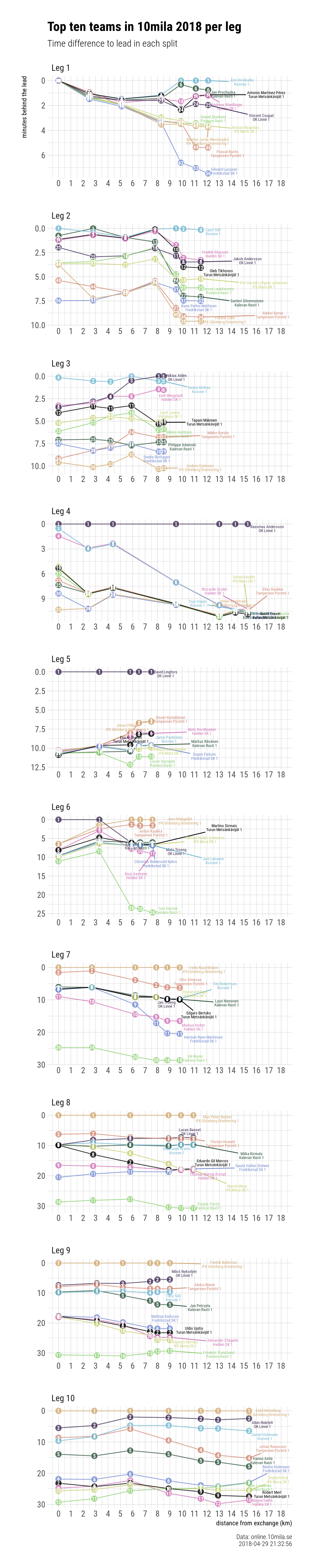
Rankings per leg at each split and at exchange

Within each leg there were three or more official split points from where you could get the data from. I took the top ten teams at finish and plotted all their runners across the ten legs. Again, OK Linne had it change, but Vetle Ruud Bråten from IFK Göteborg totally destroyed everyone else on 6th leg.

Alla olevassa kuvassa taas on kymmenen parasta joukkuetta ja niiden osuuskohtainen suorittaminen väliaikapisteiden perusteella. Linnellä oli paikka karata, mutta lopulta ratkaisun teki Göteborgin Vetle Ruud Bråten.

if (!file.exists("./data/valiaikadata.RDS")){
d_splits <- data_frame()
for (leg in 1:10){
  splits <- unlist(looptbl$splits[leg])
  split_dat <- data_frame()
  for (split1 in splits){
  read_html(paste0("http://online.10mila.se/index2.php?classId=1&legNo=",leg,"&splitNo=",split1)) %>% 
    html_table(fill = TRUE) %>% 
    .[[5]] %>% 
    .[-1:-2,] %>% 
    as_tibble() -> tmp
  names(tmp) <- c("place","name","club","time","diff")
  tmp$leg <- leg
  tmp$split1 <- split1
  split_dat <- bind_rows(split_dat,tmp)
}
  d_splits <- bind_rows(d_splits,split_dat)
}
d_splits %>% 
  mutate(
    min = as.integer(sub(":.+$", "", time)),
    s   = as.integer(sub("^.+:", "", time)),
    secs = min * 60 + s,
    diff_min = as.integer(sub(":.+$", "", diff)),
    diff_s   = as.integer(sub("^.+:", "", diff)),
    diff_secs = diff_min * 60 + diff_s
  ) -> d_splits2
saveRDS(d_splits2, "./data/valiaikadata.RDS")
}
d_splits2 <- readRDS("./data/valiaikadata.RDS")

split_info <- d_splits2 %>% count(leg,split1) %>% select(-n)
split_info %>% 
  mutate(length = case_when(
    leg == 1 & split1 ==  7 ~ 2.5,
    leg == 1 & split1 ==  8 ~ 5.1,
    leg == 1 & split1 == 10 ~ 8.3,
    leg == 1 & split1 == 11 ~ 9.9,
    leg == 1 & split1 == 12 ~ 11.1,
    
    leg == 2 & split1 == 15 ~ 2.8,
    leg == 2 & split1 == 17 ~ 5.4,
    leg == 2 & split1 == 18 ~ 7.8,
    leg == 2 & split1 == 19 ~ 9.5,
    leg == 2 & split1 == 20 ~ 10.1,

    leg == 3 & split1 == 24 ~ 2.8,
    leg == 3 & split1 == 25 ~ 4.2,
    leg == 3 & split1 == 26 ~ 5.9,
    leg == 3 & split1 == 27 ~ 8.5,

    leg == 4 & split1 == 31 ~ 2.4,
    leg == 4 & split1 == 32 ~ 4.4,
    leg == 4 & split1 == 34 ~ 9.5,
    leg == 4 & split1 == 35 ~ 13,
    leg == 4 & split1 == 36 ~ 14.3,

    leg == 5 & split1 == 39 ~ 3.3,
    leg == 5 & split1 == 40 ~ 5.8,
    leg == 5 & split1 == 42 ~ 6.5,
    
    leg == 6 & split1 == 45 ~ 3.3,
    leg == 6 & split1 == 46 ~ 5.9,
    leg == 6 & split1 == 47 ~ 6.6,

    leg == 7 & split1 == 50 ~ 2.7,
    leg == 7 & split1 == 51 ~ 6.2,
    leg == 7 & split1 == 52 ~ 7.9,
    leg == 7 & split1 == 53 ~ 8.8,

    leg == 8 & split1 == 56 ~ 2.8,
    leg == 8 & split1 == 57 ~ 5.8,
    leg == 8 & split1 == 58 ~ 8.9,
    leg == 8 & split1 == 59 ~ 9.9,

    leg == 9 & split1 == 62 ~ 3.1,
    leg == 9 & split1 == 63 ~ 5.2,
    leg == 9 & split1 == 64 ~ 7.4,
    leg == 9 & split1 == 65 ~ 8,

    leg == 10 & split1 == 68 ~ 2.9,
    leg == 10 & split1 == 70 ~ 5.8,
    leg == 10 & split1 == 71 ~ 8.9,
    leg == 10 & split1 == 72 ~ 11.5,
    leg == 10 & split1 == 73 ~ 12.9
  
  )) %>% 
  group_by(leg) %>% 
  mutate(length_cum = cumsum(length)) -> split_info

d_splits_10 <- left_join(d_splits2,split_info)

d_leg0 <- all_legs %>% filter(leg == 1) %>% mutate(length = 0, 
                                                    diff_secs = 0,
                                                    leg = 1)
d_leg_11 <- bind_rows(all_legs,d_leg_10)
d_leg_11_0 <- d_leg_11 %>% mutate(length = 0, leg = leg + 1)

legdata <- bind_rows(d_leg_11,d_leg_11_0)

d_splits_10 <- bind_rows(d_splits_10,legdata)

d_splits_10 <- d_splits_10 %>% filter(leg != 0, leg != 11)

d_splits_10$leg2 <- paste0("Leg ", d_splits_10$leg)
d_splits_10$leg2 <- factor(d_splits_10$leg2, levels = c("Leg 1","Leg 2","Leg 3","Leg 4","Leg 5","Leg 6","Leg 7","Leg 8","Leg 9","Leg 10"))

all_splits <- d_splits_10 # exceliin

d_splits_10 <- d_splits_10 %>% filter(club %in% top10)

library(ggplot2)
library(hrbrthemes)
library(viridis)
ggplot(d_splits_10, aes(x = length, y = diff_secs/60, color = club, fill = club)) + 
  geom_line(alpha = .8) + geom_point(shape = 21, color = "white", alpha = .8, size = 4) + 
  ggrepel::geom_text_repel(data = d_splits_10 %>% 
                             group_by(leg2) %>% 
                             filter(length == max(length)), 
                           aes(label = paste0(name,"\n",club)), nudge_y = -.2, nudge_x = 1, size = 2.0, lineheight = .8, family = "Roboto Condensed") + 

  facet_wrap(~leg2, ncol = 1, scales = "free") +
  scale_x_continuous(breaks = 0:18, labels = 0:18, limits = c(0,18)) +
  scale_y_reverse() + 
  geom_text(aes(label = place), color = "white", family = "Roboto Condensed", size = 2.5, fontface= "bold") +
  theme_ipsum_rc() + 
  theme(legend.position = "none") + 
  scale_fill_manual(values = c(rev(ipsum_palette),"black")) + scale_color_manual(values = c(rev(ipsum_palette),"black")) +
  # theme(plot.margin = unit(0,0,0,0)) +
  # theme(margin(t = 0, r = 0, b = 0, l = 0, unit = "pt")) +
  labs(title = "Top ten teams in 10mila 2018 per leg",
       subtitle = "Time difference to lead in each split",
       caption = paste0("Data: online.10mila.se\n",Sys.time()),
       x = "distance from exchange (km)", y = "minutes behind the lead") -> splitspic

ggsave(filename = "./kuvat/10mila2018_splits_twitter.png", splitspic, width = 6, height = 30, dpi = 120)
ggsave(filename = "./kuvat/10mila2018_splits_blogi.png", splitspic, width = 6, height = 30, dpi = 240)


# **************************************************************************************
# Omat juoksu suhteessa kärkeen

top10 <- d_leg2 %>% filter(leg == 10) %>% slice(1:10) %>% pull(club)
ourteam <- d_leg2 %>% filter(leg == 1, grepl("Veteli", club)) %>% pull(club)

top10 <- c(top10,ourteam)

d_splits_10 <- all_splits %>% filter(club %in% top10, leg == 2)

library(ggplot2)
library(hrbrthemes)
library(viridis)
ggplot(d_splits_10, aes(x = length, y = diff_secs/60, color = club, fill = club)) + 
  geom_line(alpha = .8) + geom_point(shape = 21, color = "white", alpha = .8, size = 6) + 
  ggrepel::geom_text_repel(data = d_splits_10 %>% 
                             group_by(leg2) %>% 
                             filter(length == max(length)), 
                           aes(label = paste0(name,"\n",club)), nudge_y = -.2, nudge_x = 1, size = 2.0, lineheight = .8, family = "Roboto Condensed") + 
  
  facet_wrap(~leg2, ncol = 1, scales = "free") +
  scale_x_continuous(breaks = 0:18, labels = 0:18, limits = c(0,18)) +
  scale_y_reverse() + 
  geom_text(aes(label = place), color = "white", family = "Roboto Condensed", size = 2.5, fontface= "bold") +
  theme_ipsum_rc() + 
  theme(legend.position = "none") + 
  scale_fill_manual(values = c(rev(ipsum_palette),"orange","black")) + scale_color_manual(values = c(rev(ipsum_palette),"orange","black")) +
  # theme(plot.margin = unit(0,0,0,0)) +
  # theme(margin(t = 0, r = 0, b = 0, l = 0, unit = "pt")) +
  labs(title = "My own run on leg 2 in 10mila 2018",
       subtitle = "Time difference to lead in each split, position in relay inside the dot",
       caption = paste0("Data: online.10mila.se\n",Sys.time()),
       x = "distance from exchange (km)", y = "minutes behind the lead")

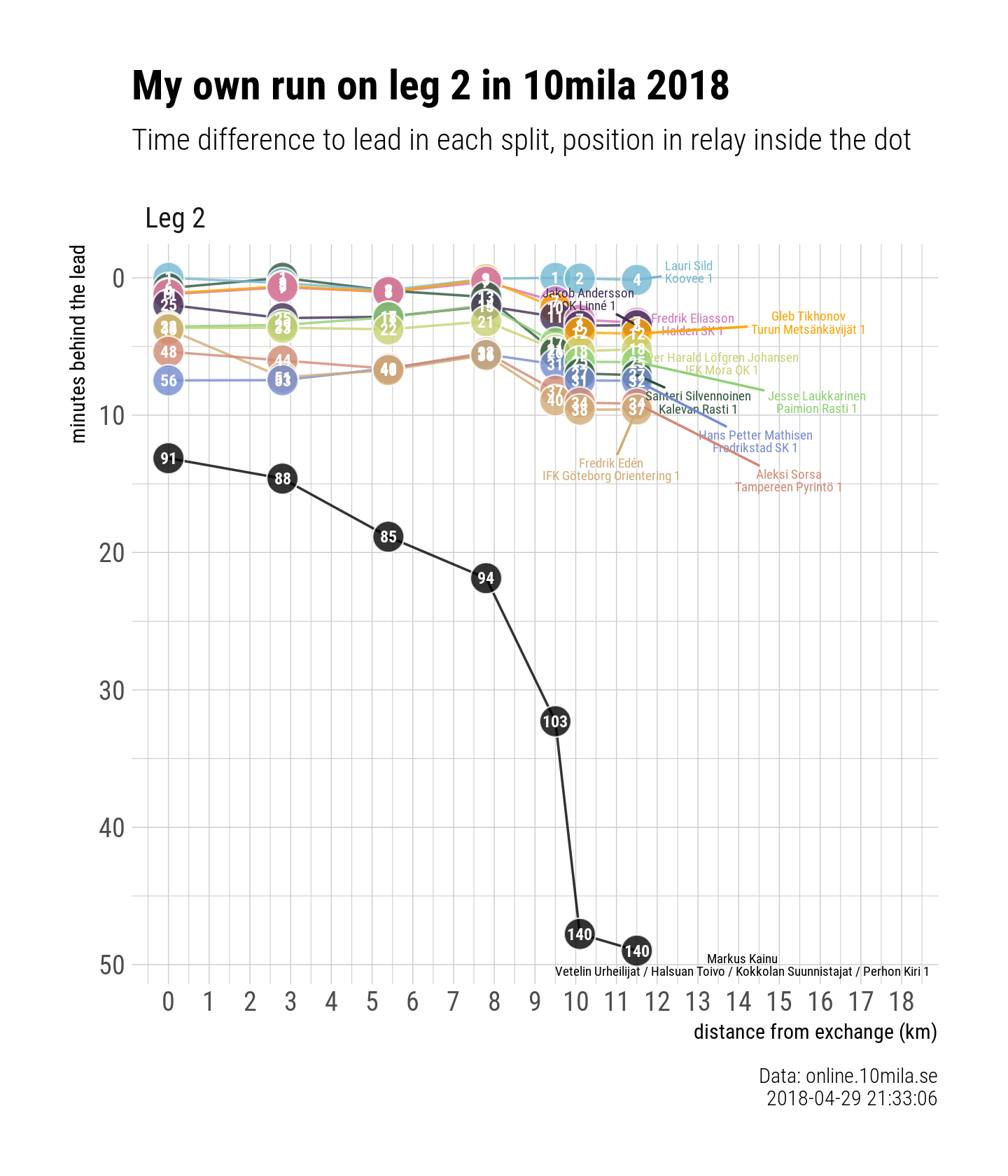
My own run

I ran the second leg in an allstars team with the best runners picked from four clubs Halsuan Toivo, Kokkolan Suunnistajat, Perhon Kiri and Vetelin Urheilijat from my home region in Finland. Our first leg runner Joonatan did a great job and I had a change to do a good run too. It started well, I kept calm and took the advantage of many top teams who were passing me after a poor first leg. Still, well after half way I felt that I am able to keep up with the pack and do a decent run. Then, after a slight calf cramp I took my own route choice, missed the control badly, had to run too fast to caught up again, missed another control.. They had left the steepest rock faces to the latter part of the course and there I completely lost my myself. Few more massive mistakes and I could only run at downhills. The plot below sums up this failure pretty well.

Six weeks to Jukola, no excuses allowed anymore.

Oma suoritus meni juuri kuin kuva näyttää. Puolenvälin yli pysyttelin mukana porukoissa, sitten pari pientä virhettä, pari isoa virhettä, pari isoa rinnettä ja viimeiset pari kilometriä kävelin. Jukolaan on kuutisen viikkoa aikaa.

top10 <- d_leg2 %>% filter(leg == 10) %>% slice(1:10) %>% pull(club)
ourteam <- d_leg2 %>% filter(leg == 1, grepl("Veteli", club)) %>% pull(club)

top10 <- c(top10,ourteam)

d_splits_10 <- all_splits %>% filter(club %in% top10, leg == 2)

library(ggplot2)
library(hrbrthemes)
library(viridis)
ggplot(d_splits_10, aes(x = length, y = diff_secs/60, color = club, fill = club)) + 
  geom_line(alpha = .8) + geom_point(shape = 21, color = "white", alpha = .8, size = 6) + 
  ggrepel::geom_text_repel(data = d_splits_10 %>% 
                             group_by(leg2) %>% 
                             filter(length == max(length)), 
                           aes(label = paste0(name,"\n",club)), nudge_y = -.2, nudge_x = 1, size = 2.0, lineheight = .8, family = "Roboto Condensed") + 
  
  facet_wrap(~leg2, ncol = 1, scales = "free") +
  scale_x_continuous(breaks = 0:18, labels = 0:18, limits = c(0,18)) +
  scale_y_reverse() + 
  geom_text(aes(label = place), color = "white", family = "Roboto Condensed", size = 2.5, fontface= "bold") +
  theme_ipsum_rc() + 
  theme(legend.position = "none") + 
  scale_fill_manual(values = c(rev(ipsum_palette),"orange","black")) + scale_color_manual(values = c(rev(ipsum_palette),"orange","black")) +
  # theme(plot.margin = unit(0,0,0,0)) +
  # theme(margin(t = 0, r = 0, b = 0, l = 0, unit = "pt")) +
  labs(title = "My own run on leg 2 in 10mila 2018",
       subtitle = "Time difference to lead in each split, position in relay inside the dot",
       caption = paste0("Data: online.10mila.se\n",Sys.time()),
       x = "distance from exchange (km)", y = "minutes behind the lead")