Analysing Transcontinental race 2022. Part 1: Data

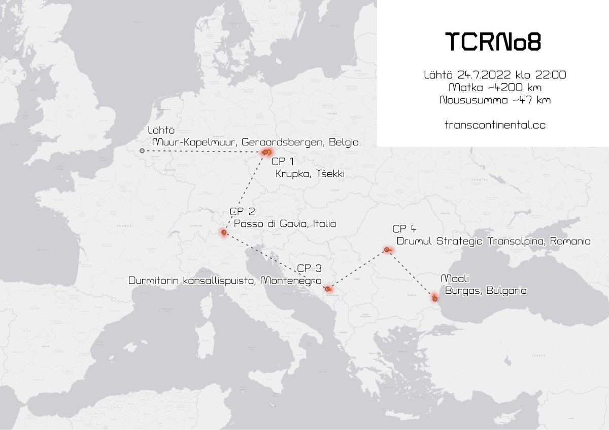
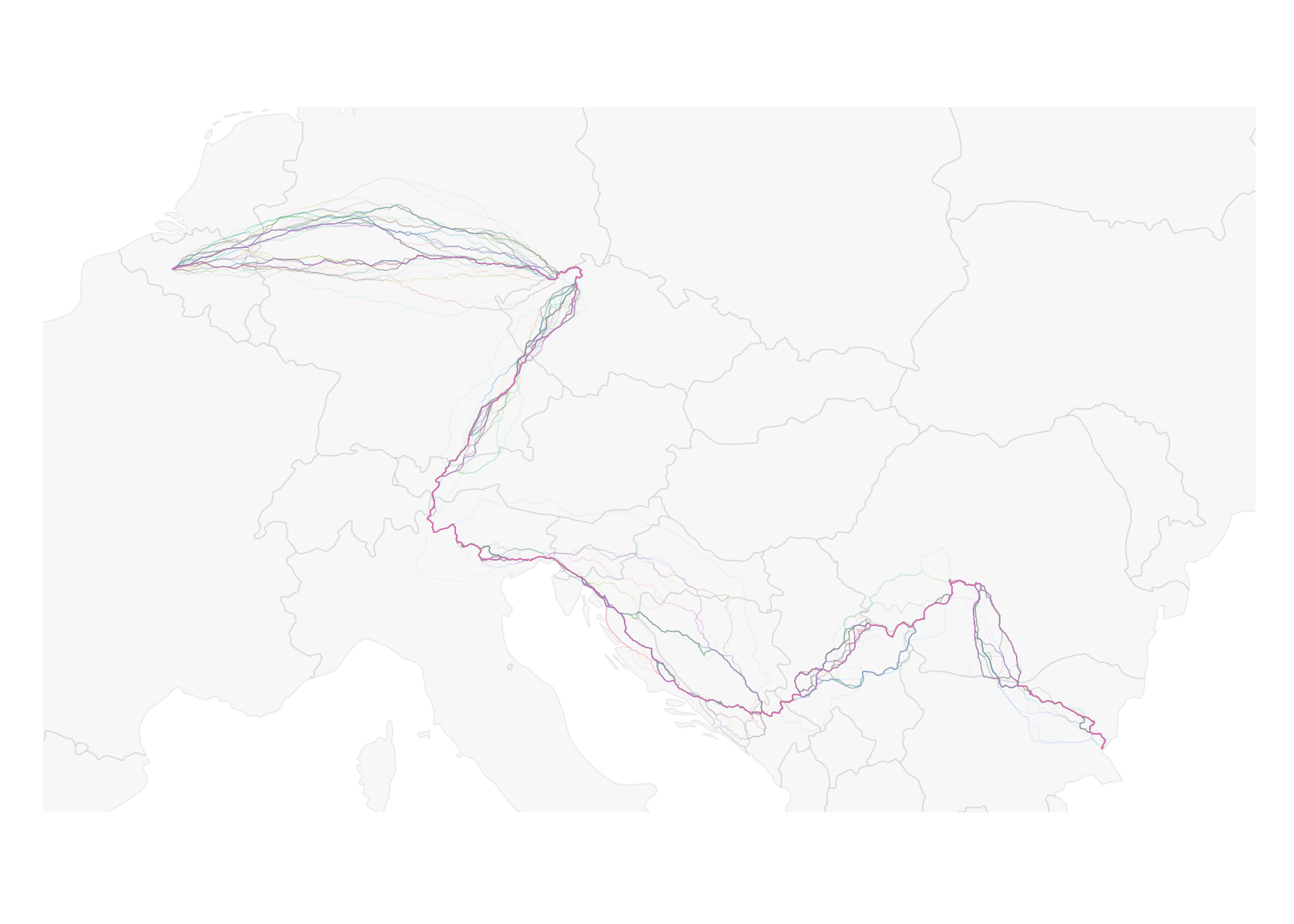
Transcontinental Race No8 (tcrno8) was ridden few weeks back in July August 2022 from Muur, Belgium to Burgas in Bulgaria. I created a “Shadow tracker” web app (not available as the race is gone) that used the data API’s of the official Follow My Challenge tracking.

This is the first part of analysis of tcrno8, and here I focus on obtaining and processing of data. I will provide code snippets in R-language for you to reproduce.

Tärkeää

Follow My Challenge does not provide details on their data licencing and therefore I won’t share any data here, only code!

Replay data from Follow my Challenge

Follow my Challenge has a replay mode for replaying the race afterwards. Replay mode displays data that is available at https://www.followmychallenge.com/live/tcrno8/data/replaydata.js and can be processed R sf -object (points) with code below.

library(jsonlite)
library(dplyr)
library(sf)
library(ggplot2)

# Route data
lns <- readLines("https://www.followmychallenge.com/live/tcrno8/data/replaydata.js")

lns[1] <- sub('var replay_', '{"', lns[1])
lns4 <- gsub('var replay_', '"', lns) %>%
  gsub(' = ', '":', .) %>%
  gsub("]}};", "]}},", .)
lns5 <- lns4[-length(lns4)]
lns5[length(lns5)] <- sub(",", "}", lns5[length(lns5)])
dat <- fromJSON(lns5)

dat_lst <- list()
nms <- names(dat)
for (i in seq(nms)){
  tmp_lst <- dat[[nms[i]]]
  coord <- tmp_lst$geometry$coordinates
  tmp_dat <- tibble(lon = coord[,1], lat = coord[,2],
                time = as.POSIXct(tmp_lst$properties$time,  origin="1970-01-01")) %>%
    st_as_sf(coords=c("lon","lat"), crs=4326) %>% 
    mutate(riderName = tmp_lst$properties$name,
           teamNumber = tmp_lst$properties$teamNumber)
  dat_lst[[i]] <- tmp_dat
}
routes <- do.call("rbind", dat_lst)

Raw spatial data from tracking looks like this.

plot(routes[,"riderName"])

Attribute data from tracking

Real-time mode in Follow my challenge show additional data from each rider such as distance ridden, time since last report, current speed or scratcing status. The data from the latest location can be accessed in here https://www.followmychallenge.com/live/tcrno8/data/ridersArray.json. This data also has the altitude value for that particular point, but we don’t need it as we sourced it elsewhere for the replay data.

With the following code we can get the latest tracking data and join that with longitudinal replay data.

# Attribute data
urli <- "https://www.followmychallenge.com/live/tcrno8/data/ridersArray.json"
d <- fromJSON(txt = url(urli))
nms_single <- c("riderName", 
                "country",
                "scratched",
                "teamNumber",
                "groupHeaderLabel",
                "movingTimePercentage",
                "totalDistance",
                "finishTime")

dlist <- list()
for (i in 1:length(d)){
  tmp <- d[[i]]
  nms <- names(tmp)
  tmp_lst <- list()
  for (ii in seq(nms_single)){
    nm2 <- nms_single[[ii]]
    tmp_lst[[nm2]] <- tmp[[nm2]]
  }
  tmp_df1 <- as.data.frame(tmp_lst) %>% as_tibble()
  dlist[[i]] <- tmp_df1
}
df <- do.call("bind_rows", dlist) 
# head(df)

Finally we will join the few new variable from attribute data with our replay data.

routes_and_points <- left_join(routes,df)
glimpse(routes_and_points)

Rows: 487,161
Columns: 10
$ time                 <dttm> 2022-07-24 23:00:00, 2022-07-24 23:06:37, 2022-0…
$ geometry             <POINT [°]> POINT (3.88277 50.7716), POINT (3.87354 50.…
$ riderName            <chr> "Marin de Saint-Exupéry", "Marin de Saint-Exupéry…
$ teamNumber           <chr> "42", "42", "42", "42", "42", "42", "42", "42", "…
$ country              <chr> "France.png", "France.png", "France.png", "France…
$ scratched            <int> 0, 0, 0, 0, 0, 0, 0, 0, 0, 0, 0, 0, 0, 0, 0, 0, 0…
$ groupHeaderLabel     <chr> "Solo", "Solo", "Solo", "Solo", "Solo", "Solo", "…
$ movingTimePercentage <int> 78, 78, 78, 78, 78, 78, 78, 78, 78, 78, 78, 78, 7…
$ totalDistance        <dbl> 4586.8, 4586.8, 4586.8, 4586.8, 4586.8, 4586.8, 4…
$ finishTime           <chr> "1659558856", "1659558856", "1659558856", "165955…

Dropping riders with sparse data

Tärkeää

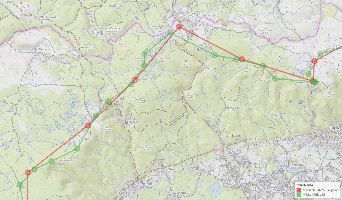
Replay data from Follow my route is far from perfect. There seems to be some systematic missing data from some riders, and not just due to scratching, but perhaps some device/hardware issue.

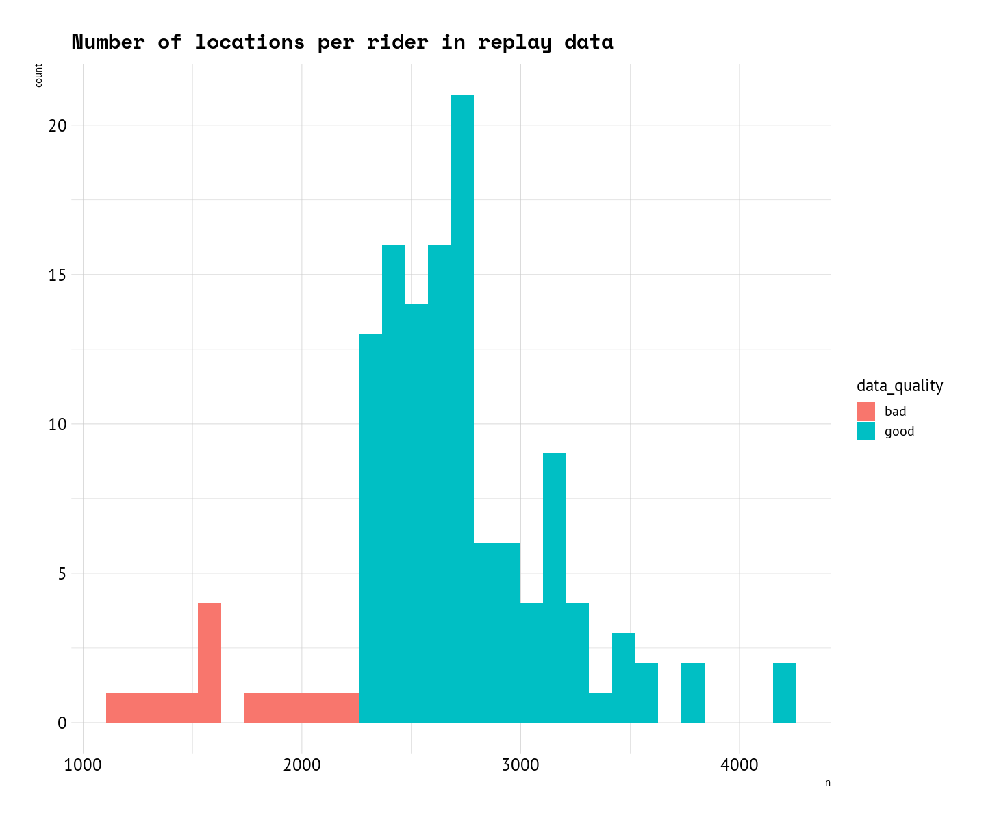
To solve this I will exclude two groups or riders: 1) scratched and 2) one with less than 2250 location points in the data.

First group is obvious, second one is based on the a breaking point in the distribution of location points. As shown in the plot below, majority of the riders have more than 2250 location points (labelled as “good” quality data). Including riders with few location points will affect the more detailed route choice or resting pattern analyses.

routes_and_points %>% 
  st_drop_geometry() %>% 
  filter(scratched == 0) %>% 
  count(riderName) %>% 
  arrange(n)  -> nr_logs
# reactable::reactable(nr_logs, searchable = TRUE)
nr_logs_d <- nr_logs %>% 
  mutate(data_quality = ifelse(n > 2250, "good", "bad"))

ggplot(nr_logs_d, aes(x = n, fill = data_quality)) + 
  geom_histogram() + 
  labs(title = "Number of locations per rider in replay data")

# 
# top5 <- nr_logs_d %>% 
#     filter(data_quality == "bad") %>% 
#     pull(riderName) %>% .[1:5]
# 
# p2 <- ggplot(routes_and_points %>% 
#                filter(riderName %in% top5), 
#              aes(color = riderName)) + 
#   geom_sf() + 
#   labs(title = "Top 5 finished riders with fewest data points",
#        subtitle = "all excluded from analysis")
# wrap_plots(list(p1,p2), heights = c(1.2,.8), ncol = 1)

To be pricise, the following riders will be excluded from the analysis due to bad data quality.

nr_logs_d %>% 
    filter(data_quality == "bad") %>% 
    pull(riderName)

 [1] "Max Riese"              "Marin de Saint-Exupéry" "Andrew Dumbill"        
 [4] "Meaghan Hackinen"       "Paolo Laureti"          "Wouter Van der Hallen" 
 [7] "Nico Coetzee"           "Douglas Migden"         "Rob Leslie"            
[10] "Joseph Dorsett"         "Krisjanis Ratiniks"     "Fiona Kolbinger"       

And here is a close-up showing how the data quality issue looks in real world.

Adding elevation

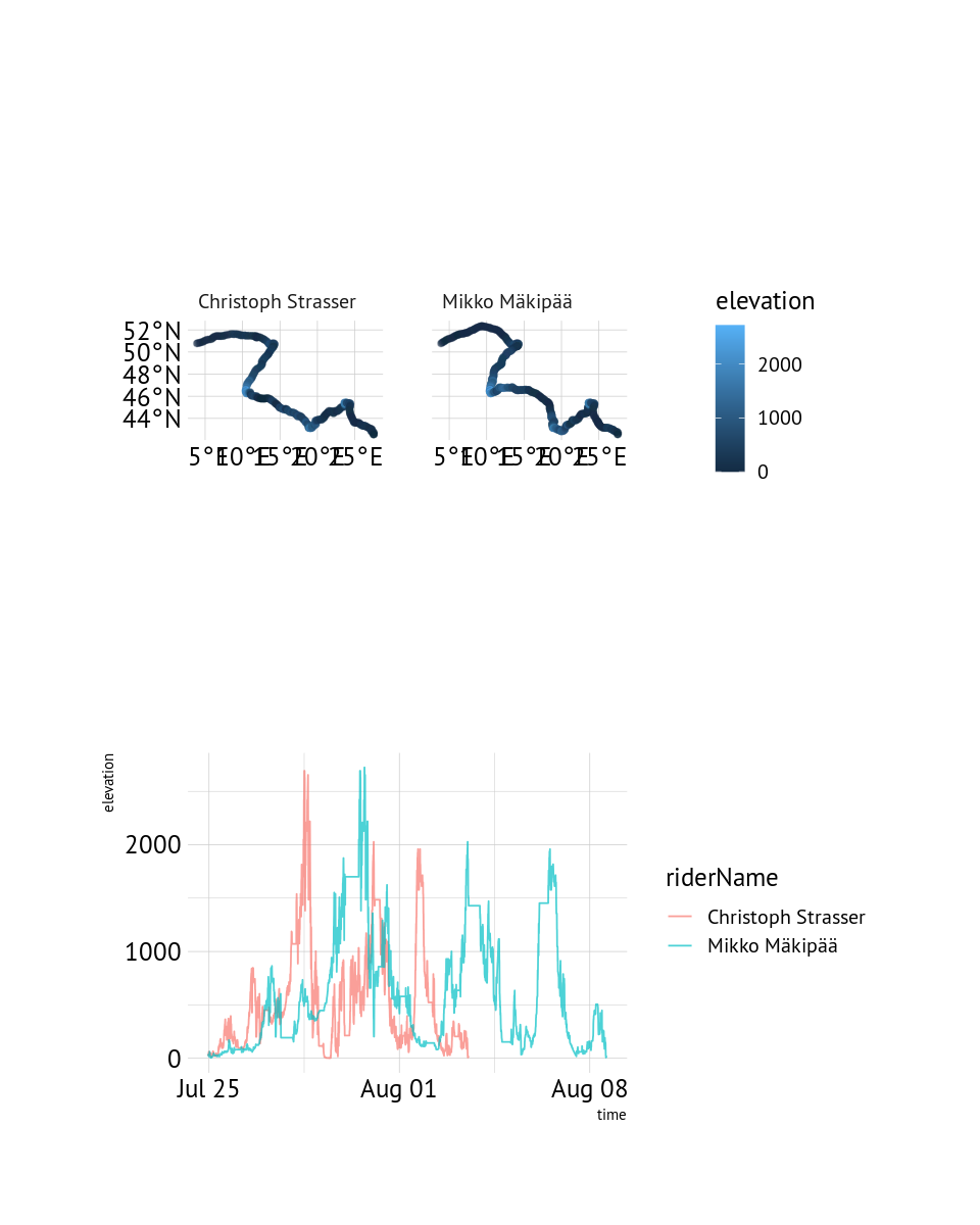
Replay data only show point location in lat/lon with time, but is missing elevation. elevatr provides functions to inteface with AWS terrain tiles to get elevation data for any location point. It is straightforward to add elevation for each location.

dat_all_points2 <- routes_and_points %>% 
  left_join(nr_logs_d %>% select(riderName,data_quality))
library(elevatr)
dat_all_points <- get_elev_point(dat_all_points2, src = "aws")

As a results, we can plot Mikko Mäkipää’s and Christoph Strassers altitude data both as spatial data and as a function of time.

dat_all_points %>% 
  filter(grepl("Mäkipää|Strasser", riderName)) -> mpaa
ggplot(mpaa, aes(color = elevation)) +
  theme(legend.position = "right") + facet_wrap(~riderName) +
  geom_sf(alpha = .1) -> p
ggplot(st_drop_geometry(mpaa), aes(x = time, y = elevation, color = riderName)) +
  geom_line(alpha = .7) + theme(legend.position = "right") -> p2
library(patchwork)
wrap_plots(list(p,p2), heights = c(1.2,.8), ncol = 1)

Plotting the cleaned route data

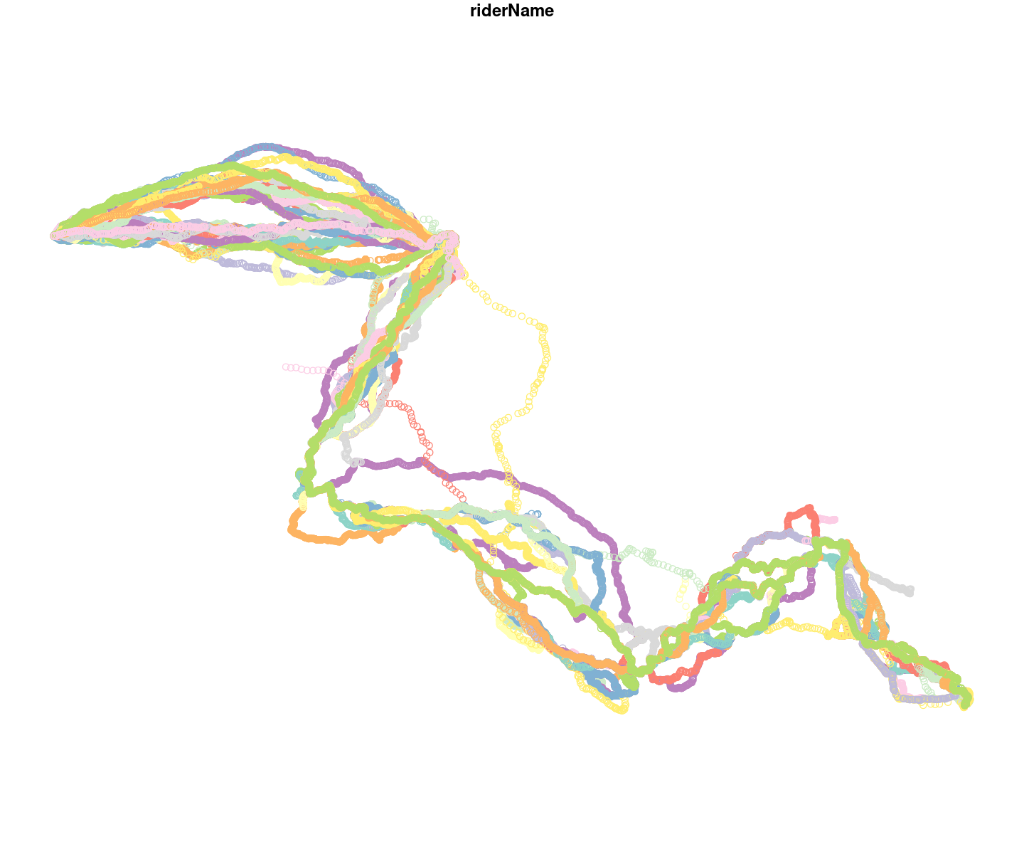
As a final step in this data sourcing post, we will transform the POINT data with 330693 rows in into MULTILINESTRING data with single row per rider, containing only the riders that did not scratch and whose location data is of “good quality”.

dat_all_linestring <- dat_all_points %>% 
group_by(riderName) %>% 
  filter(scratched == 0,
         data_quality == "good") %>%
  summarize(m = mean(row_number()),
            teamNumber = teamNumber[1],
            country = country[1],
            groupHeaderLabel = groupHeaderLabel[1],
            movingTimePercentage = movingTimePercentage[1],
            totalDistance = max(totalDistance),
            finishTime = min(finishTime),
            do_union=FALSE) %>%
  st_cast("MULTILINESTRING") %>% 
  arrange(finishTime)

Finally, with this route data, we can draw a plot with routes of all riders who made it through the race.

cntry <- rnaturalearthdata::countries50
cntry_sf <- st_as_sf(cntry) %>% 
  filter(subregion %in% c("Southern Europe",
                          "Western Europe",
                          "Eastern Europe"))

ggplot(dat_all_linestring,
       aes(color = riderName)) +
  geom_sf(data = cntry_sf, 
          color = alpha("dim grey", 1/10), 
          fill = alpha("dim grey", 1/20)) +
  geom_sf(alpha = .1,size = .3) + 
  ylim(c(42,53)) +
  xlim(c(2,30)) +
  theme(legend.position = "none",
        panel.grid.major = element_blank(),
        axis.text.x = element_blank(),
        axis.text.y = element_blank()
        )

In next few parts we will analyse the route choices and resting patterns of riders.